Topical Articles

Bayesian CNN via TFP vs CNN

This was introduced by Blundell et al (2015) and then adopted by many researchers in recent years.

Non-Bayes trains point estimate of weights
Bayes approximates distribution of weights commonly basing on Gaussian (mean, sd), prior and data
- Prediction via posterior distribution of weights
- So far, there are several existing packages in Python that implement Bayesian CNN. For example, Shridhar et al 2018used Pytorch (also see their blogs), Thomas Wiecki 2017 used PyMC3, and Tran et al 2016 introduced the package Edward and then merged into TensorFlow Probability (Tran et al 2018).

DEMO: Single-node CNN as baseline

import os
import warnings
# warnings.simplefilter(action="ignore")
warnings.filterwarnings('ignore')
os.environ['TF_CPP_MIN_LOG_LEVEL'] = '3'
import matplotlib.pyplot as plt
from matplotlib import figure 
from matplotlib.backends import backend_agg
import seaborn as sns
from tensorflow.examples.tutorials.mnist import input_data
import tensorflow as tf
import numpy as np
tf.logging.set_verbosity(tf.logging.ERROR)
# Dependency imports
import matplotlib
import tensorflow_probability as tfp
matplotlib.use("Agg")
%matplotlib inline

# data
mnist_onehot = input_data.read_data_sets(data_dir, one_hot=True)
mnist_conv = input_data.read_data_sets(data_dir,reshape=False ,one_hot=False)
mnist_conv_onehot = input_data.read_data_sets(data_dir,reshape=False ,one_hot=True)
# display an image
img_no = 485
one_image = mnist_conv_onehot.train.images[img_no].reshape(28,28)
plt.imshow(one_image, cmap='gist_gray')
print('Image label: {}'.format(np.argmax(mnist_conv_onehot.train.labels[img_no])))

# baseline effectively multinomial logistic reg
# define placeholders
x = tf.placeholder(tf.float32, shape=[None, 28*28])
y_true = tf.placeholder(tf.float32, shape=[None, 10])
# define variables: weights and bias
W = tf.Variable(tf.zeros([28*28, 10]))
b = tf.Variable(tf.zeros([10]))
# create graph operations
y = tf.matmul(x,W)+b
# define loss function
cross_entropy = tf.reduce_mean(tf.nn.softmax_cross_entropy_with_logits(labels=y_true, logits=y))
# define optimizer
optimizer = tf.train.GradientDescentOptimizer(learning_rate=0.5)
train=optimizer.minimize(cross_entropy)
# create session
epochs = 5000
init = tf.global_variables_initializer()
with tf.Session() as sess:
    sess.run(init)
    for step in range(epochs):
        batch_x, batch_y = mnist_onehot.train.next_batch(50)
        sess.run(train, feed_dict={x:batch_x, y_true:batch_y})
    
    #EVALUATION
    correct_preds = tf.equal(tf.argmax(y,1), tf.argmax(y_true, 1))
    acc = tf.reduce_mean(tf.cast(correct_preds, tf.float32))
    
    print('Accuracy on test set: {}'.format(
        sess.run(acc, feed_dict={x: mnist_onehot.test.images, y_true: mnist_onehot.test.labels})))
    
# CNN
# Conv(32), MaxPooling, Conv(64), MaxPooling, Flatten, Dense(1024), Dropout(50%), Dense(10)
x = tf.placeholder(tf.float32,shape=[None,28,28,1])
y_true = tf.placeholder(tf.float32,shape=[None,10])
hold_prob = tf.placeholder(tf.float32)
cnn = tf.keras.Sequential()
cnn.add(tf.keras.layers.Conv2D(32, kernel_size=5, padding='SAME', activation=tf.nn.relu))
cnn.add(tf.keras.layers.MaxPooling2D(pool_size=[2, 2], strides=[2, 2], padding="SAME"))
cnn.add(tf.keras.layers.Conv2D(64, kernel_size=5, padding='SAME', activation=tf.nn.relu))
cnn.add(tf.keras.layers.MaxPooling2D(pool_size=[2, 2], strides=[2, 2], padding="SAME"))
cnn.add(tf.keras.layers.Flatten())
cnn.add(tf.keras.layers.Dense(1024, activation=tf.nn.relu))
cnn.add(tf.keras.layers.Dropout(hold_prob))
cnn.add(tf.keras.layers.Dense(10))
y_pred = cnn(x)
cross_entropy = tf.reduce_mean(tf.nn.softmax_cross_entropy_with_logits(labels=y_true,logits=y_pred))
optimizer = tf.train.AdamOptimizer(learning_rate=0.0001)
train = optimizer.minimize(cross_entropy)
steps = 5000
init = tf.global_variables_initializer()
with tf.Session() as sess:
    sess.run(init)
    
    for i in range(steps+1):
        batch_x , batch_y = mnist_conv_onehot.train.next_batch(50)
        sess.run(train,feed_dict={x:batch_x,y_true:batch_y,hold_prob:0.5})
        
        # PRINT OUT A MESSAGE EVERY 100 STEPS
        if i%500 == 0:
            matches = tf.equal(tf.argmax(y_pred,1),tf.argmax(y_true,1))
            acc = tf.reduce_mean(tf.cast(matches,tf.float32))
            print('Step {}: accuracy={}'.format(i, sess.run(acc,feed_dict={x:mnist_conv_onehot.test.images,                 y_true:mnist_conv_onehot.test.labels,                                                                           hold_prob:1.0})))

Bayesian CNN

TFP GitHub Code

images = tf.placeholder(tf.float32,shape=[None,28,28,1])
labels = tf.placeholder(tf.float32,shape=[None,])
hold_prob = tf.placeholder(tf.float32)
# define the model
neural_net = tf.keras.Sequential([
      tfp.layers.Convolution2DReparameterization(32, kernel_size=5,  padding="SAME", activation=tf.nn.relu),
      tf.keras.layers.MaxPooling2D(pool_size=[2, 2],  strides=[2, 2],  padding="SAME"),
      tfp.layers.Convolution2DReparameterization(64, kernel_size=5,  padding="SAME",  activation=tf.nn.relu),
      tf.keras.layers.MaxPooling2D(pool_size=[2, 2], strides=[2, 2], padding="SAME"),
      tf.keras.layers.Flatten(),
      tfp.layers.DenseFlipout(1024, activation=tf.nn.relu),
      tf.keras.layers.Dropout(hold_prob),
      tfp.layers.DenseFlipout(10)])
logits = neural_net(images)
# Compute the -ELBO as the loss, averaged over the batch size.
labels_distribution = tfp.distributions.Categorical(logits=logits)
neg_log_likelihood = -tf.reduce_mean(labels_distribution.log_prob(labels))
kl = sum(neural_net.losses) / mnist_conv.train.num_examples
elbo_loss = neg_log_likelihood + kl
optimizer = tf.train.AdamOptimizer(learning_rate=learning_rate)
train_op = optimizer.minimize(elbo_loss)
# Build metrics for evaluation. Predictions are formed from a single forward
# pass of the probabilistic layers. They are cheap but noisy predictions.
predictions = tf.argmax(logits, axis=1)
accuracy, accuracy_update_op = tf.metrics.accuracy(labels=labels, predictions=predictions)

learning_rate = 0.001   #initial learning rate
max_step = 5000 #number of training steps to run
batch_size = 50 #batch size
viz_steps = 500 #frequency at which save visualizations.
num_monte_carlo = 50 #Network draws to compute predictive probabilities.
init_op = tf.group(tf.global_variables_initializer(),
                     tf.local_variables_initializer())

with tf.Session() as sess:
        sess.run(init_op)
# Run the training loop.
        for step in range(max_step+1):
            images_b, labels_b = mnist_conv.train.next_batch(
batch_size)
            images_h, labels_h = mnist_conv.validation.next_batch(
mnist_conv.validation.num_examples)
            
            _ = sess.run([train_op, accuracy_update_op], feed_dict={
                   images: images_b,labels: labels_b,hold_prob:0.5})
        if (step==0) | (step % 500 == 0):
                loss_value, accuracy_value = sess.run([elbo_loss, accuracy], feed_dict={images: images_b,
labels: labels_b,hold_prob:0.5})
                
                print("Step: {:>3d} Loss: {:.3f} Accuracy: {:.3f}".format(step, loss_value, accuracy_value))

Structural Time Series Modeling via TFP

Intro to tfp.sts , a new lib for forecasting time series using structural time series models.

sts models comprise a family of proba-ts generalising:

AR process
MA
Local Linear Trends
Seasonality
Regression and variable selection on external covariates (other TS might related to the series of interest)

A STS model expresses an observed TS as sum of simpler components:

$f(t) = f_1(t) + f_2(t) + … + f_n(t) + \varepsilon~;~\varepsilon~\thicksim~N(0, \sigma^2) $

Each component governed by a particular structural basis, e.g. one encoding seasonal effect (day-week), another local linear trend, yet another linear dependence on some set of covariate TS

By allowing modelers to encode assumptions about the processes generating the data, structural time series can often produce reasonable forecasts from relatively little data (e.g., just a single input series with tens of points). The model’s assumptions are interpretable, and we can interpret the predictions by visualizing the decompositions of past data and future forecasts into structural components. Moreover, structural time series models use a probabilistic formulation that can naturally handle missing data and provide a principled quantification of uncertainty.

TFP integration with built-in Bayesian inference of model parameters using VI and HMC, computing both point forecasts and predictive uncertainties, empowered by TF ecosystem on hardware

import tensorflow_probability as tfp
trend = tfp.sts.LocalLinearTrend(observed_time_series=co2_by_month)
seasonal = tfp.sts.Seasonal(
	num_seasons=12, observed_time_series=co2_by_month)
model = tfp.sts.Sum([trend, seasonal], observed_time_series=co2_by_month)

The full code for this example is available on Github.

Next we’ll consider a more complex example: forecasting electricity demand in Victoria, Australia. The top line of this plot shows an hourly record from the first six weeks of 2014 (data from [4], available at https://github.com/robjhyndman/fpp2-package):

Electricity

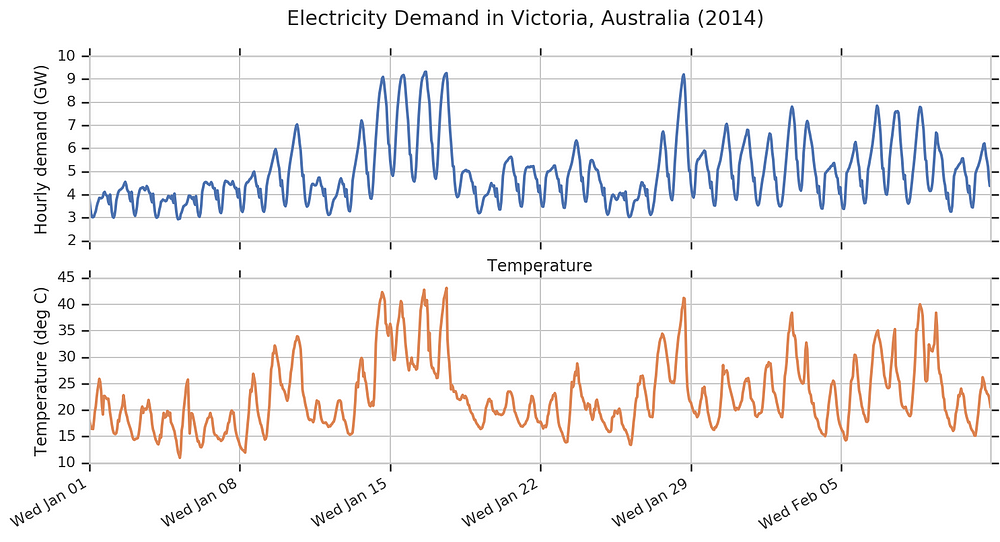
external source of info: temperature, correlating with electricity demand for air conditioning, incorporated in STS model via linear regression

temperature_effect = tfp.sts.LinearRegression(
	design_matrix=tf.reshape(temperature - np.mean(temperature),
                          (-1, 1)), name='temperature_effect')
hour_of_day_effect = tpf.sts.Seasonal(
	num_season=24,
	observed_time_series=demand,
	name='hour_of_day_effect')
day_of_week_effect = tfp.sts.Seasonal(
  num_seasons=7,
  num_steps_per_season=24, 
  observed_time_series=demand,
  name='day_of_week_effect')
residual_level = tfp.sts.Autoregressive(
  order=1,
  observed_time_series=demand, name='residual')
model = tfp.sts.Sum([temperature_effect,
                     hour_of_day_effect,
                     day_of_week_effect,
                     residual_level],
                    observed_time_series=demand)

also included multiple seasonal effects and AR component to model any unexplained residual effects - could use simple random walk, but chose an AR for keeping bounded variance over time

Results

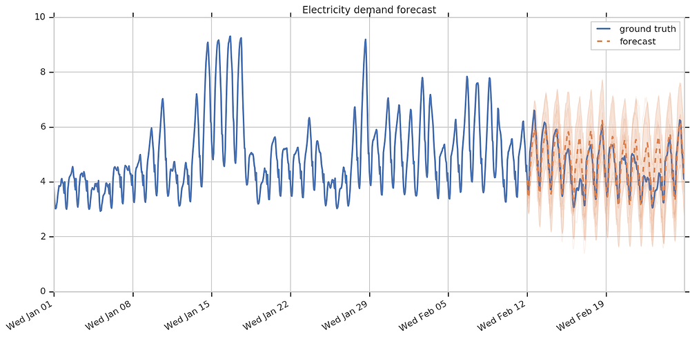
apparently still some unmodeled sources of variation

model reasonably captured seasonal effect and sizable external temperature effect with confident forecasts but less so on AR
might further improve via spikes in temperature seemingly coinciding with spikes in AR residual - indicating additional features or data transformations might help çapture temperature effect!!

The full code for this example is available on Github.

TFP STS Library

STS is a linear model on additive components such as:
- Autoregressive, LocalLinearTrend, SemiLocalLinearTread, and LocalLevel. For modeling time series with a level or slope that evolves according to a random walk or other process.
- Seasonal. For time series depending on seasonal factors, such as the hour of the day, the day of the week, or the month of the year.
- LinearRegression. For time series depending on additional, time-varying covariates. Regression components can also be used to encode holiday or other date-specific effects.
STS provides methods for fitting the resulting time series models with variational inference and Hamiltonian Monte Carlo.

[1] Brodersen, K. H., Gallusser, F., Koehler, J., Remy, N., & Scott, S. L. (2015). Inferring causal impact using Bayesian structural time-series models. The Annals of Applied Statistics, 9(1), 247–274.

[2] Choi, H., & Varian, H. (2012). Predicting the present with Google Trends. Economic Record, 88, 2–9.

[3] Harvey, A. C. (1989). Forecasting, structural time series models and the Kalman filter. Cambridge University Press.

[4] Hyndman, R.J., & Athanasopoulos, G. (2018). Forecasting: principles and practice, 2nd edition, OTexts: Melbourne, Australia. OTexts.com/fpp2. Accessed on February 23, 2019.